The perceptron algorithm is a basic machine learning architecture which can classify linearly separable data by learning an accurate model from training data. Understanding the perceptron algorithm is key in understanding neural networks. This article will explain the perceptron algorithm and how it works.
Imagine a university accepts candidates based on their grades and their entrance exam scores, and we want to build a model which will accurately predict whether a candidate is accepted based on past data.
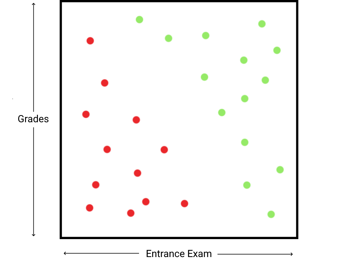
There are two input variables, \(x_g\) and \(x_e\), where \(0 \le x_g, x_e \le 100\). We want to find some function \(f(\overrightarrow{x})\), where \(\overrightarrow{x}\) is the vector of inputs, that separates the input data into rejected and accepted categories.
To classify the data, let's assign values above 0 as being accepted and values below 0 being rejected. As the data is linearly separable, our target function can be modelled linearly. This means we can define the following equation for \(f(\overrightarrow{x})\):
$$\displaylines{f(\overrightarrow{x}) = ax_g + bx_e + c\\a,b,c \in \mathbb{R}}$$
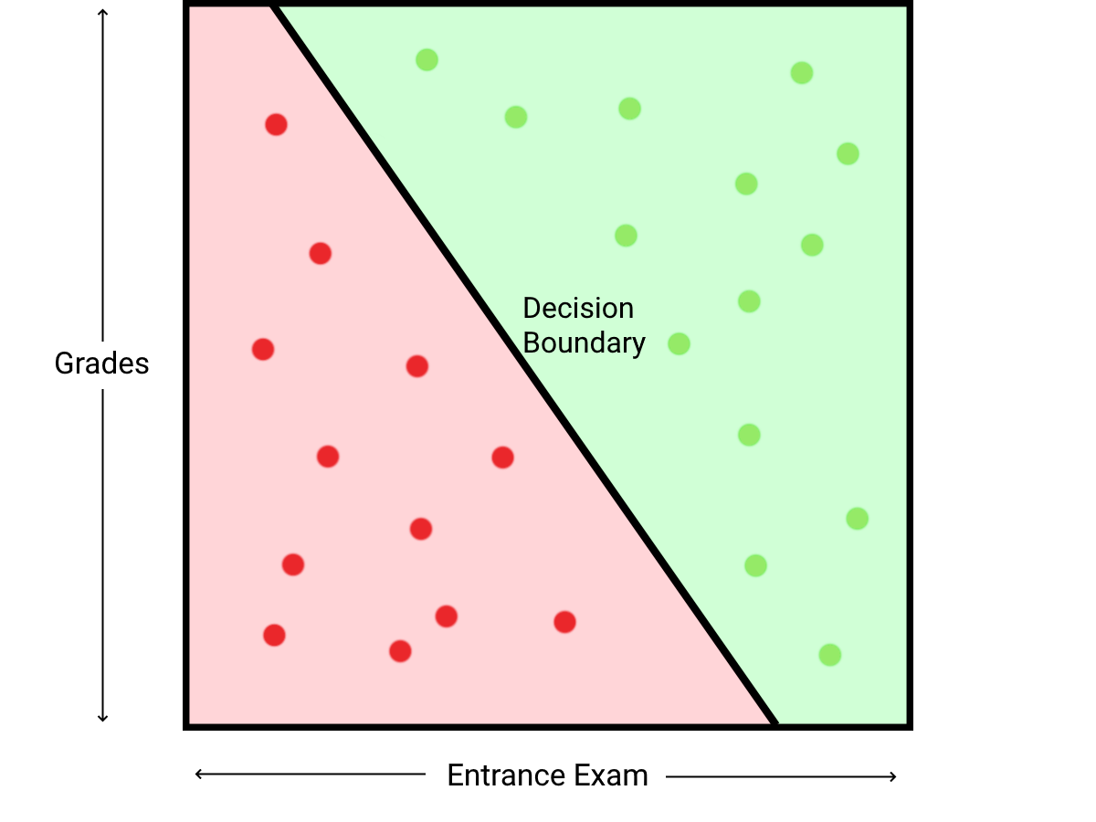
We can find the decision boundary of the equation, which is where \(f(x) = 0\). This divides the problem space into two sections, one for rejected inputs, and one for accepted inputs. To convert our continuous output into a binary output, the heaviside step function can be used to convert positive numbers to 1 and negative numbers to 0.
Despite this problem being trivial when solved graphically, solving the problem programmatically can be more challenging. However, gradient descent can be used to solve this problem. By iteratively improving the initial parameters of the function, gradient descent converges to better parameters which will produce a more accurate model.
Let's initialise our desired function \(f(\overrightarrow{x})\) with unoptimised parameters \(a=1\), \(b=1\), \(c=-10\). $$f(\overrightarrow{x}) = x_e + x_g - 10$$ This will accept any person who gets over 10% total, which will not accurately classify the data. We can input a rejected student with a 15% average in their results and 55% on the entrance exam and see that they're incorrectly classified. $$\displaylines{f(\overrightarrow{x_1}) = 55 + 15 - 10 = 60 \\ H(f(\overrightarrow{x_1})) = H(60) = 1}$$
where H(x) is the heaviside step function.
An output of 1 means these results would be accepted by the current function. As we have labeled data and a current output of the model, we know which direction we want the output of this model to move. The parameters of the function need to be tuned such that the function outputs a lower value. This can be achieved by differentiating the function and finding the rate of change of the output with respect to each parameter, we then know the effect of each parameter on the output and know how much to change them to approach the target. This technique is known as gradient descent.
As the function uses multiple parameters we must use partial differentiation to find the rates of change for each parameter, which is where all other parameters are treated as constants. The partial derivative is denoted by \(\frac{\partial y}{\partial x}\). $$\frac{\partial f(\overrightarrow{x})}{\partial a} = \frac{\partial}{\partial a}ax_e + bx_g + c$$ $$= \frac{\partial}{\partial a}ax_e + D$$ $$= x_e$$ It turns out that the rate of change of the output with respect to the \(a\) parameter is the exams result. As the function returned a value which was too high, we can subtract this rate of change from the parameter. This will lower the output of the function, which will bring the output closer to the desired value.
Each step of gradient descent involves taking a small step in the direction of a better result.
These steps allow us to optimise our function by shifting the parameters with each incorrect classification over many samples. $$a = a - \frac{\partial f(\overrightarrow{x_1})}{\partial a}$$ $$\frac{\partial f(\overrightarrow{x_1})}{\partial a} = 55$$ $$a = 1 - 55 = -54$$
We can find our new values for the \(b\) and \(c\) parameters as well by subtracting the partial derivative of \(f(\overrightarrow{x})\) with respect to each parameter.
$$b = b - \frac{\partial f(\overrightarrow{x_1})}{\partial b}$$ $$\frac{\partial f(\overrightarrow{x_1})}{\partial b} = \frac{\partial}{\partial b}ax_e + bx_g + c$$ $$= \frac{\partial}{\partial b}bx_g + D$$ $$= x_g$$ $$b = b - x_g$$ $$b = 1 - 15 = -14$$
$$c = c - \frac{\partial f(\overrightarrow{x_1})}{\partial c}$$ $$\frac{\partial f(\overrightarrow{x_1})}{\partial c} = \frac{\partial}{\partial c}ax_e + bx_g + c$$ $$= \frac{\partial}{\partial c}c + D$$ $$= 1$$ $$c = c - 1$$ $$c = 10 - 1 = 9$$
If this is repeated over multiple training examples, an optimal decision boundary can be found, where every point in the training data is correctly classified. These steps define the perceptron algorithm, and it is proven that the algorithm will always converge to an optimal solution if the data is linearly separable.
Usually each adjustment is multiplied by some fraction known as the 'learning rate'. This allows the algorithm to converge smoothly, making it easier to find precise parameters.
Through these steps we have implemented a basic machine learning algorithm, allowing the program to solve the problem with no knowledge of the problem domain besides the classification of the training data. The perceptron algorithm is only able to classify linearly separable data, however it is used as a building block in neural networks which can solve much more complex problems.