Neural networks are one of the most important architecures in machine learning and are used ubiquitously in modern AI. This article will cover how the most common neural network (the multilayer perceptron) learns and the motivation behind some characteristics of its design. It builds upon my article on perceptrons.
The perceptron can only classify a limited number of datasets. The simplest problem which a perceptron cannot be trained to solve is an XOR function.
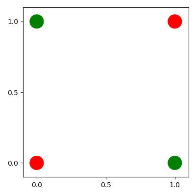
There is no line which will separate the green and red classes, so a perceptron will never converge.
To classify this data, we need to train a model which is able to output non-linear decision boundaries. This is because the data is not linearly separable. To allow the model to output non-linear decision boundaries, we need to change the architecture of the perceptron. This gives the motivation behind the multilayer perceptron.
To understand multilayer perceptrons, we must first change our visualisation of the perceptron. Previously, the output of the perceptron was defined as \(H(ax_1 + bx_2 + c)\). We can rewrite this in vector notation as follows: $$H(\begin{pmatrix} x_1\\x_2 \end{pmatrix} \cdot \begin{pmatrix} a\\b \end{pmatrix} + c)$$ The heaviside step function checks if the output is larger than 0, so we can shift the \(c\) parameter across to get an equivalent expression: $$\begin{pmatrix} x_1\\x_2 \end{pmatrix} \cdot \begin{pmatrix} a\\b \end{pmatrix} > -c$$ We have now expressed our output in terms of a threshold activation, where the output is only 1 if the vector dot product is larger than \(-c\). The model can now be visualised graphically.
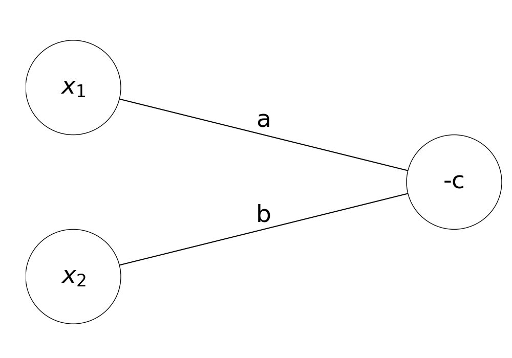
Our nodes in this graph are called neurons, the parameters multiplying each input are called weights and the threshold activation, or bias, is the parameter inside the output neuron. This visualisation makes it easy to graph multilayer perceptrons, so now we can design one which can solve the XOR problem.
We can split our XOR problem into multiple linearly separable problems as follows:
\((1):\) Is at least one of the inputs activated? (OR)
\((2):\) Are both of the inputs activated? (AND)
\((3):\) Is \((1)\) true and \((2)\) false? (XOR)
By using multiple layers of perceptrons, we can combine these into one model.
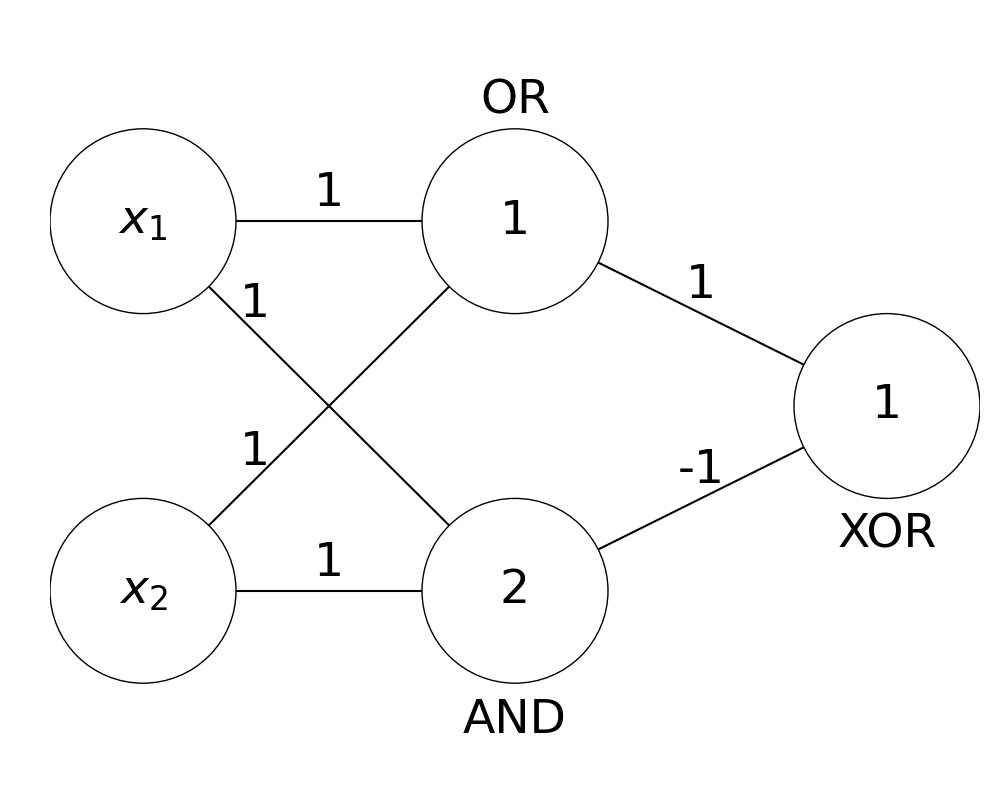
Note: here the threshold activations are shown as the lowest integers at which the neuron will activate.
By dividing the non-linear XOR function into linear components, we have found a model which is able to classify the XOR function successfully. In fact, using a multilayer perceptron and dividing a problem into multiple linearly separable problems is able to approximate any arbitrary continuous function, as shown in the universal approximation theorem.
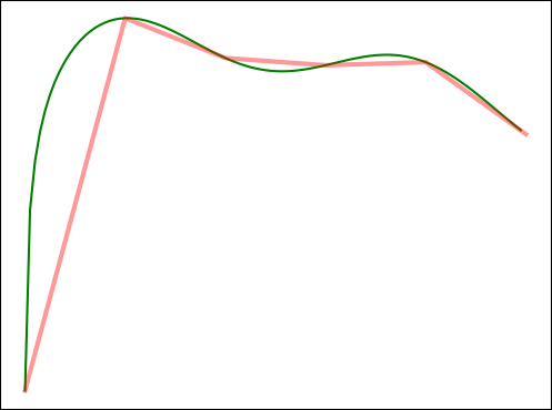
Any continuous function can be approximated by a multilayer perceptron.
Theoretically, we now have a model powerful enough to classify any continuous relationship in data. However, we haven't yet covered how to learn parameters to solve non-linear classification problems. Similarly to perceptrons, gradient descent can be used to find these parameters.
To use gradient descent, the derivative of the output with respect to each parameter must be calculated. Then, this rate of change can be used to shift the parameter to approach a target output. As an example, we can use a model of the same size as the previous example.
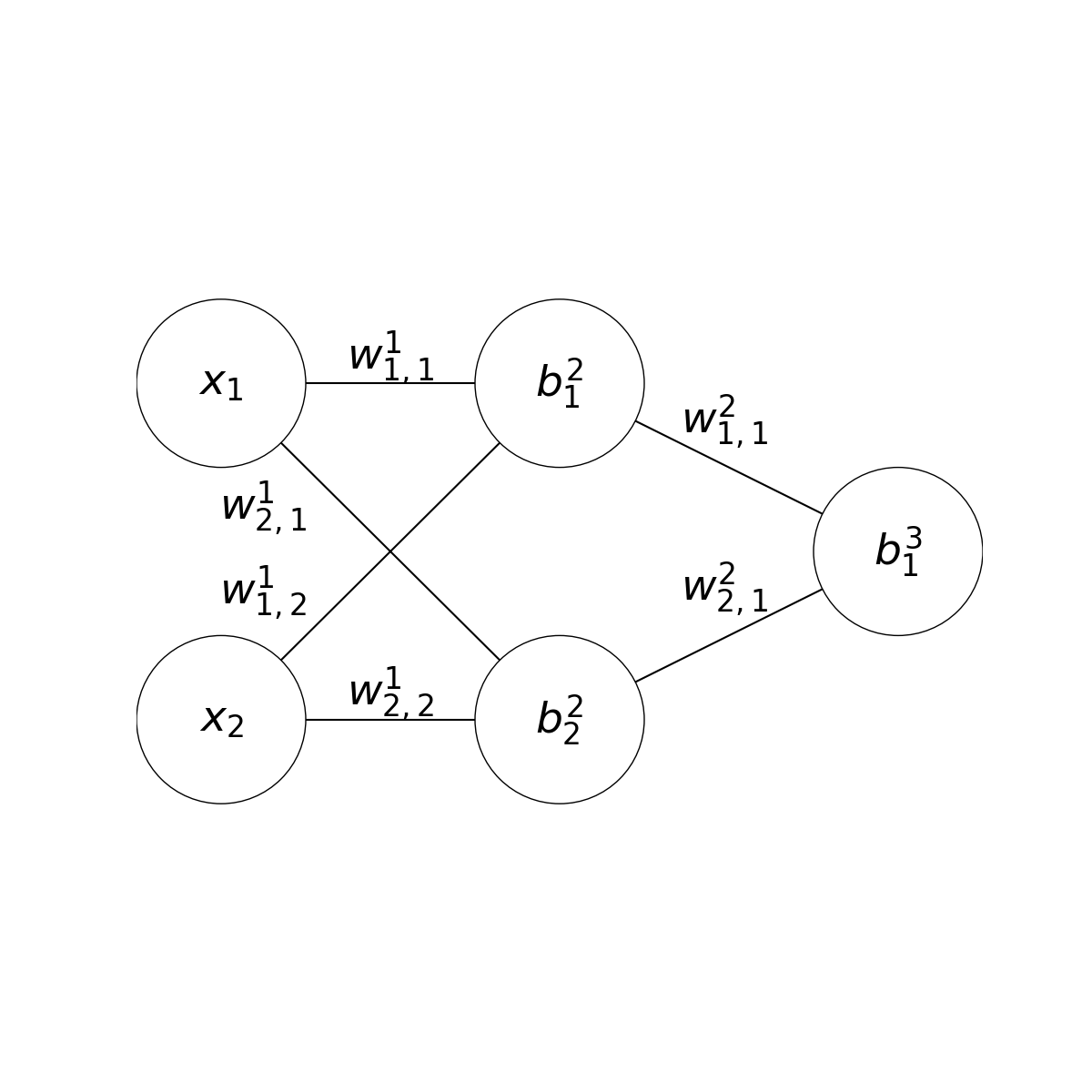
I will now refer to the parameters as \(w^i_{j,k}\) for the weight connecting the \(j\)th neuron in the \(i\)th layer with the \(k\)th neuron in the next layer, and \(b^i_j\) for the bias of the \(j\)th neuron in the \(i\)th layer. Additionally, \(a^i_j\) is typically used to denote the activation, or value, of the \(j\)th neuron in the \(i\)th layer.
If we focus on the last two layers, we can see that they form a perceptron. This means the last layer of parameters can be differentiated in the same way as before. $$f(\overrightarrow{x}) = (w^2_{1,1} \cdot a^2_1) + (w^2_{2,1} \cdot a^2_2) + b^3_1$$
$$\frac{\partial}{\partial w^2_{1,1}} f(\overrightarrow{x})$$ $$= \frac{\partial}{\partial w^2_{1,1}} (w^2_{1,1} \cdot a^2_1) + C$$ $$= a^2_1$$
$$\frac{\partial}{\partial w^2_{2,1}} f(\overrightarrow{x})$$ $$= \frac{\partial}{\partial w^2_{2,1}} (w^2_{2,1} \cdot a^2_2) + C$$ $$= a^2_2$$
$$\frac{\partial}{\partial b^3_1} f(\overrightarrow{x})$$ $$= \frac{\partial}{\partial b^3_1} C$$ $$= 1$$
In models with many neurons and layers, there is the possibility of each parameter affecting the output through multiple paths in the network. To account for this, we can use a differentiation technique known as backpropagation.
By using the chain rule we can split our derivatives into manageable parts. By finding the rate of change of the output with respect to each neuron \((\frac{\partial f(\overrightarrow{x})}{\partial a^i_j})\), you can work backwards and calculate the derivatives for the weights and biases.
$$\frac{\partial f(\overrightarrow{x})}{\partial w^1_{1,1}} = \frac{\partial f(\overrightarrow{x})}{\partial a^2_1} \cdot \frac{\partial a^2_1}{\partial w^1_{1,1}}$$
$$\frac{\partial f(\overrightarrow{x})}{\partial a^2_1}$$ $$= \frac{\partial}{\partial a^2_1} (w^2_{1,1} \cdot a^2_1) + (w^2_{2,1} \cdot a^2_2) + b^3_1$$ $$= \frac{\partial}{\partial a^2_1} (w^2_{1,1} \cdot a^2_1) + C$$ $$= w^2_{1,1}$$
$$\frac{\partial a^2_1}{\partial w^1_{1,1}}$$ $$= \frac{\partial}{\partial w^1_{1,1}} (w^1_{1,1} \cdot a^1_1) + (w^1_{2,1} \cdot a^1_2) + b^2_1$$ $$= \frac{\partial}{\partial w^1_{1,1}} (w^1_{1,1} \cdot a^1_1) + C$$ $$= a^1_1$$
$$\frac{\partial f(\overrightarrow{x})}{\partial w^1_{1,1}} = w^2_{1,1} \cdot a^1_1$$
This finds how much the weight/bias affects the neuron, and how much the neuron affects the output. When multiplied, this gives the rate of change of the output with respect to the weight/bias. This technique is known as backpropagation and allows for more complex derivatives to be computed. However, this omits a crucial step: the activation function.
The non-linearity of a multi-layer perceptron is caused by some activation function, which is applied to each weighted sum \(z\) to get the output of the neuron. So far we have used a threshold activation to introduce this non-linearity. However, this function is not differentiable, so it cannot be used in backpropagation. Instead, we can use a sigmoid function.
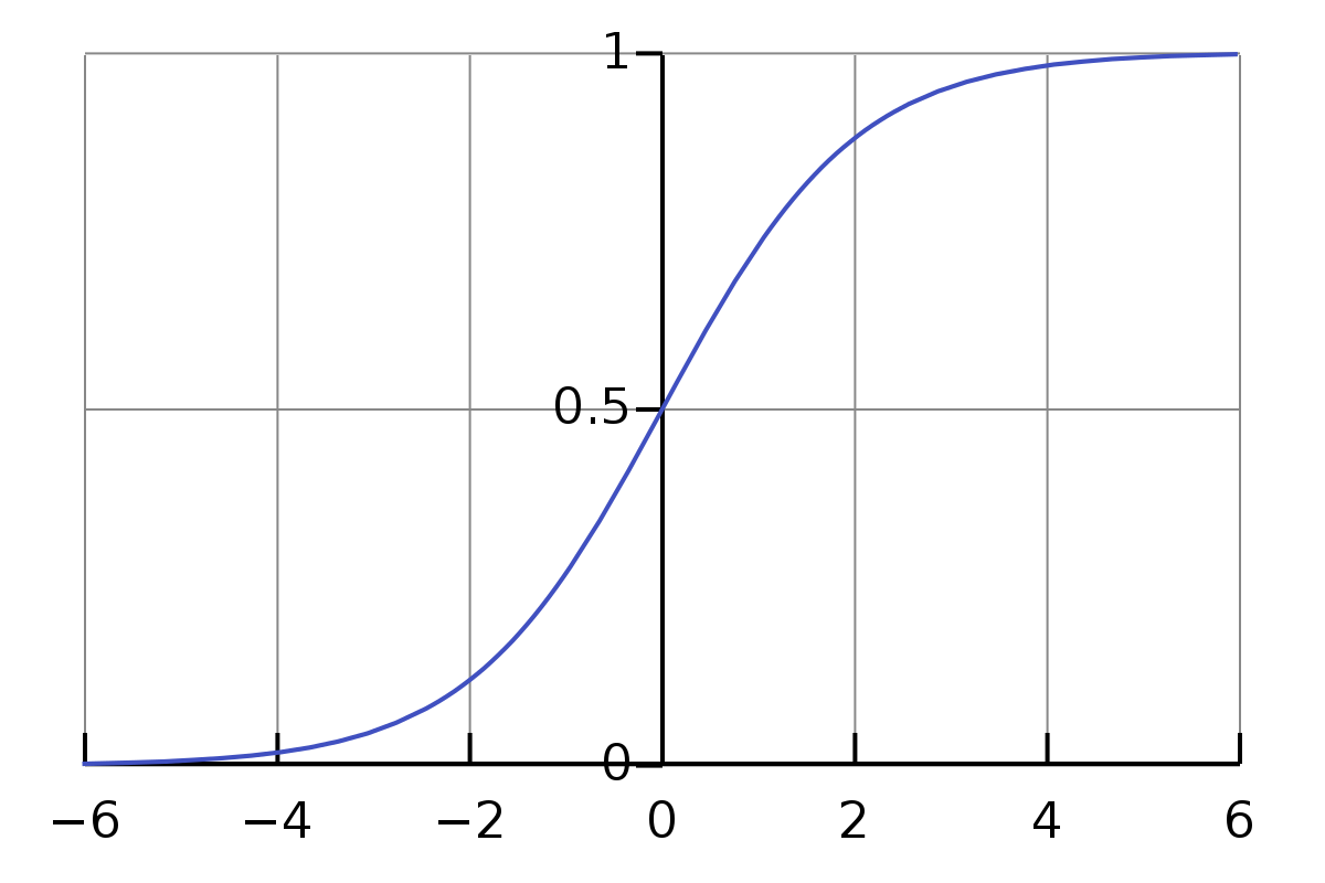
The sigmoid function \(\sigma(x)\) restricts the output to the range \([0, 1]\).
$$\sigma(x) = \frac{1}{1 + e^{-x}}$$
The activation function is applied to the weighted sum of the inputs to get the output of the neuron.
$$z^{i+1}_j = w^i_{1,j} \cdot a^i_1 + ... + w^i_{n,j} \cdot a^i_n + b^{i+1}_j)$$
$$a^{i+1}_j = \sigma(z^{i+1}_j)$$
However, as this function affects the activation of the neuron, it also affects the derivative of the neuron, so it must be included in the backpropagation. To simplify the equation, let's refer to the rate of change of the output with respect to a particular neuron \(a^i_j\) as \(\delta^i_j\), or the error of the neuron.
$$\delta^i_j = \frac{\partial f(\overrightarrow{x})}{\partial a^i_j}$$
$$\delta^i_j = \delta^{i+1}_1 \cdot \frac{\partial a^{i+1}_1}{\partial a^i_j} + ... + \delta^{i+1}_n \cdot \frac{\partial a^{i+1}_n}{\partial a^i_j}$$
This line states that the error of a neuron is defined by how much it affects the output of the next layer, and how much the next layer affects the output of the model.
$$\frac{\partial a^{i+1}_1}{\partial a^i_j} = \frac{\partial a^{i+1}_1}{\partial z^{i+1}_j} \cdot \frac{\partial z^{i+1}_j}{\partial a^i_j}$$
Then, we can use the chain rule to split the derivative of the activation function into its parts.
$$\frac{\partial a^{i+1}_1}{\partial z^{i+1}_j}$$ $$= \frac{\partial}{\partial z^{i+1}_j} \sigma(z^{i+1}_j)$$ $$= \sigma(z^{i+1}_j) \cdot (1 - \sigma(z^{i+1}_j))$$ $$= a^{i+1}_1 \cdot (1 - a^{i+1}_1)$$
$$\frac{\partial z^{i+1}_j}{\partial a^i_j}$$ $$= \frac{\partial}{\partial a^i_j} (w^i_{1,j} \cdot a^i_1) + ... + (w^i_{n,j} \cdot a^i_n) + b^{i+1}_j$$ $$= w^i_{1,j}$$
$$\frac{\partial a^{i+1}_1}{\partial a^i_j} = a^{i+1}_1 \cdot (1 - a^{i+1}_1) \cdot w^i_{1,j}$$
$$\delta^i_j = \delta^{i+1}_1 \cdot a^{i+1}_1 \cdot (1 - a^{i+1}_1) \cdot w^i_{1,j} + ... + \delta^{i+1}_n \cdot a^{i+1}_n \cdot (1 - a^{i+1}_n) \cdot w^i_{n,j}$$
Click on a section of the network to backpropagate.
By iterating through our dataset and adjusting the parameters of the network using backpropagation, we approach a network which classifies the data correctly.
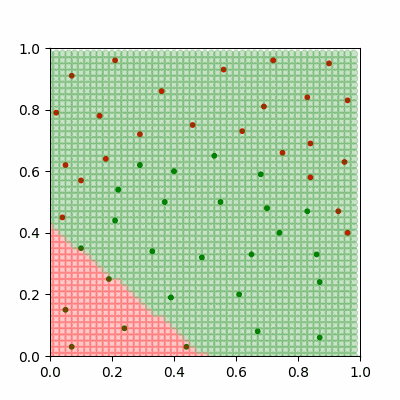
A neural network learning to classify non-linear data.
These steps give us a very powerful model which can learn complex relationships in data over time, however it is unable to solve problems where our data might be in more than two categories. If we need more classes then we must change our model slightly.
If we want to classify the MNIST dataset of hand-drawn digits, a great dataset for a first attempt at neural networks, we should give our model 10 neurons in the output layer, with each neuron representing the model's confidence of the input image representing each digit.
To allow backpropagation to work on these non-binary problems, we can define a cost function C.
$$C(\overrightarrow o) = \frac{1}{10} \sum_{i=1}^{10} (o_i - d_i)^2$$
The cost function defines how far away the output of the network is from the desired output. An easy cost function to use is the mean squared error (MSE) of the output layer of the network \(o\) compared to the desired outputs \(d\). In this case the desired output is 1 for the correct digit and 0 for incorrect digits. We want to minimise the cost function, and can accomplish this by finding the rate of change of the cost function with respect to each parameter. If we find how much each output neuron affects the cost function, we can adjust our parameters in the same way as before.
$$\frac{\partial C(\overrightarrow o)}{\partial o_i} = \frac{\partial}{\partial o_i} \cdot \frac{1}{10}(o_i-d_i)^2$$
$$= \frac{1}{10} \cdot 2(o_i-d_i)$$
$$= \frac{1}{5}(o_i-d_i)$$
$$\delta^L_i = \frac{1}{5}(o_i-d_i)$$
This new error in the last layer can be backpropagated to minimise the cost function. Each parameter now finds the rate of change of the cost function with respect to itself.
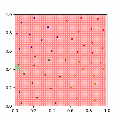
A neural network with four classes. The source code for this network is linked below.