Convolutional neural networks (CNNs) are vital in processing images using machine learning. CNNs use spatial locality to simplify images and successfully classify them with a small network size. This article assumes knowledge from my article on neural networks.
The multi-layer perceptron is not a good architecture for image classification. Every neuron in a multi-layer perceptron is connected to every neuron in the next layer, so when processing an image with millions of pixels and 3 colour channels as an input, the number of parameters becomes intractable.
By passing over the input with a small filter, the network learns to extract features of the image. Convolutional neural networks are able to process images with a small number of parameters, and are therefore good choices for image processing.
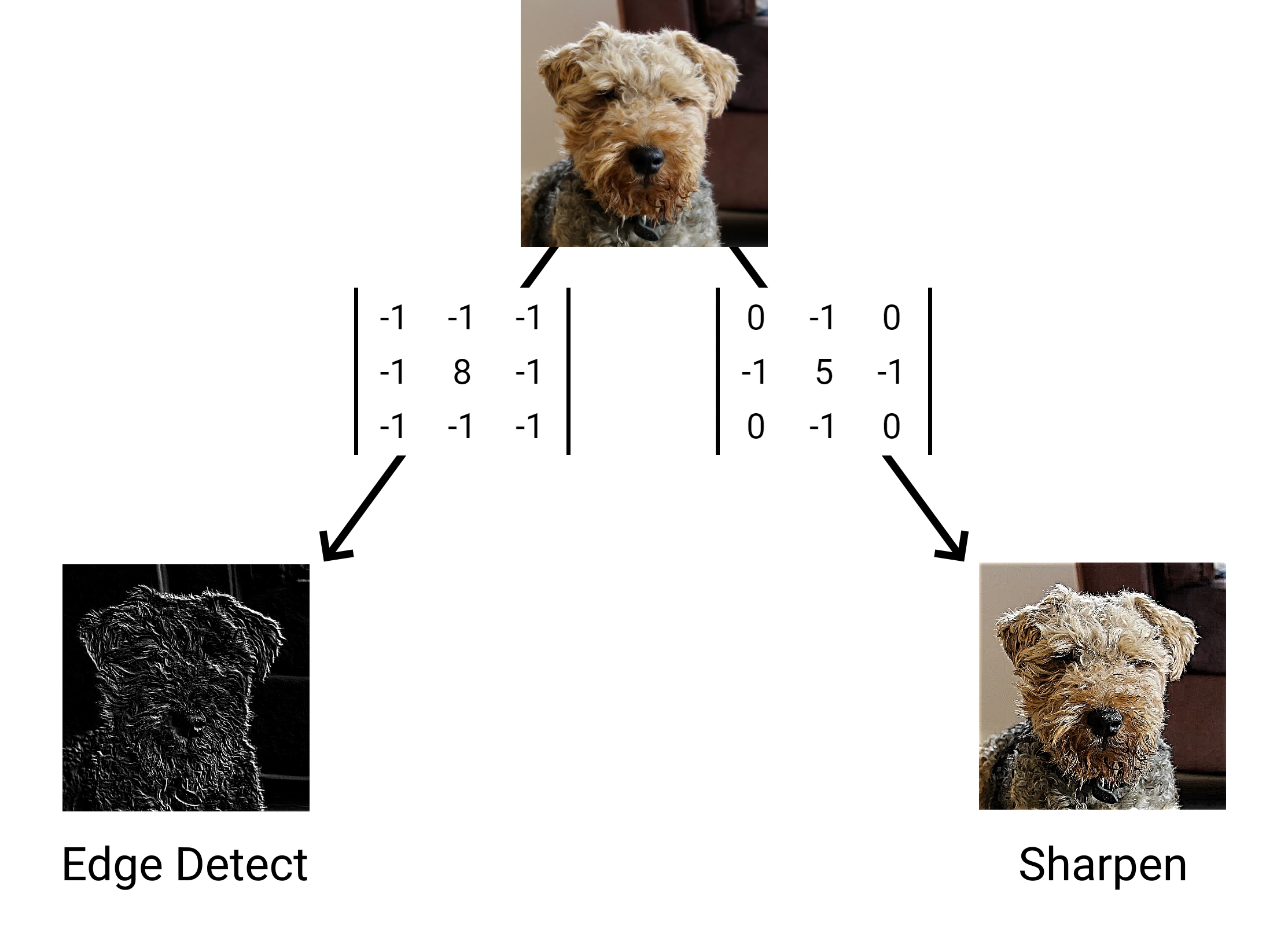
Convolutional neural networks rely on the ability for a matrix to be able to extract useful features from an image. This is shown to be possible by image filters such as edge detection and sharpening, which work by using a matrix to convolve over an image.
As shown above, as little as 9 parameters can successfully extract a feature from an image. As convolutions can extract certain features (such as edges), it is reasonable to assume a machine learning algorithm could extract arbitrary features by learning its own filter matrices. Convolutional neural networks use this assumption to learn appropriate filters to extract relevant features for a classification task.
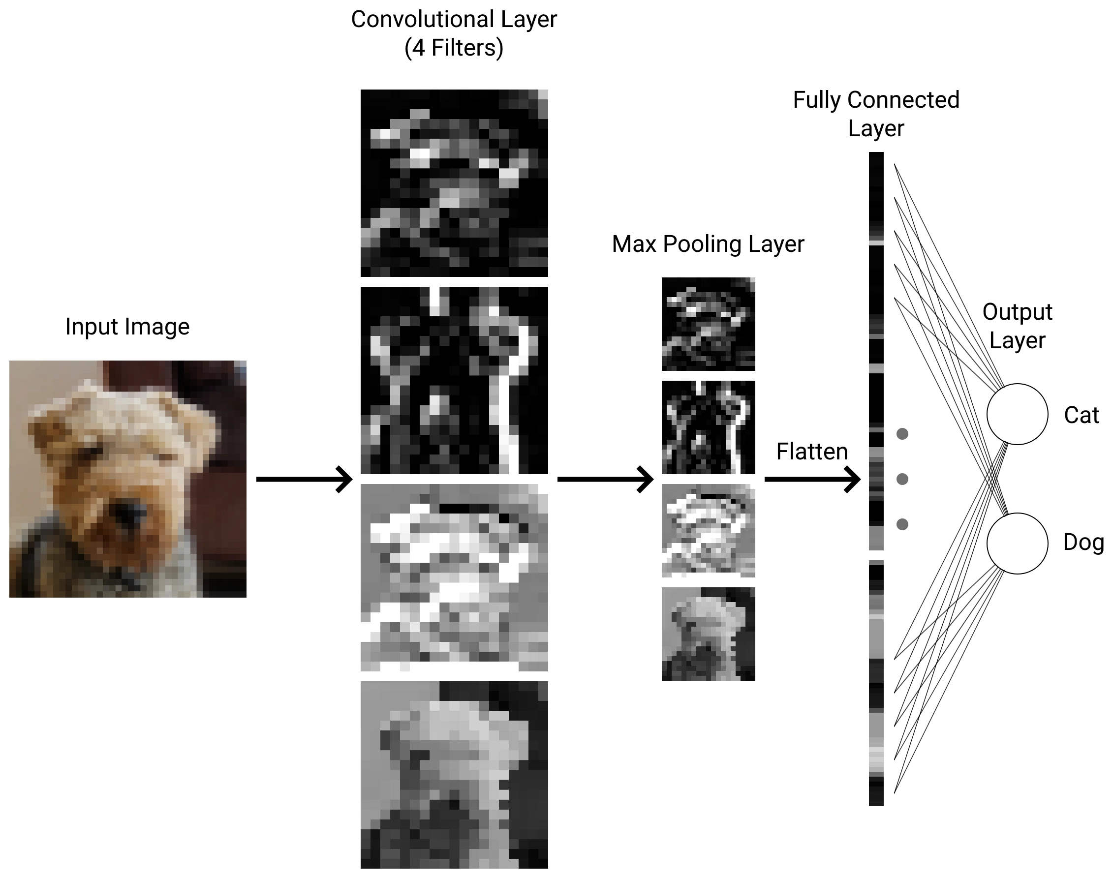
A CNN is composed of several layers, the most important being the convolutional layer. The convolutional layer is responsible for applying filters over the input.
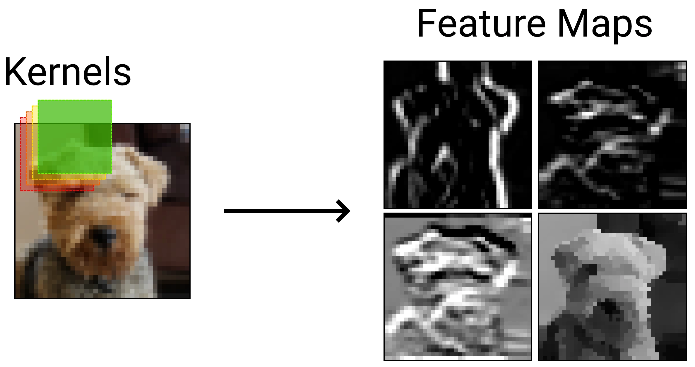
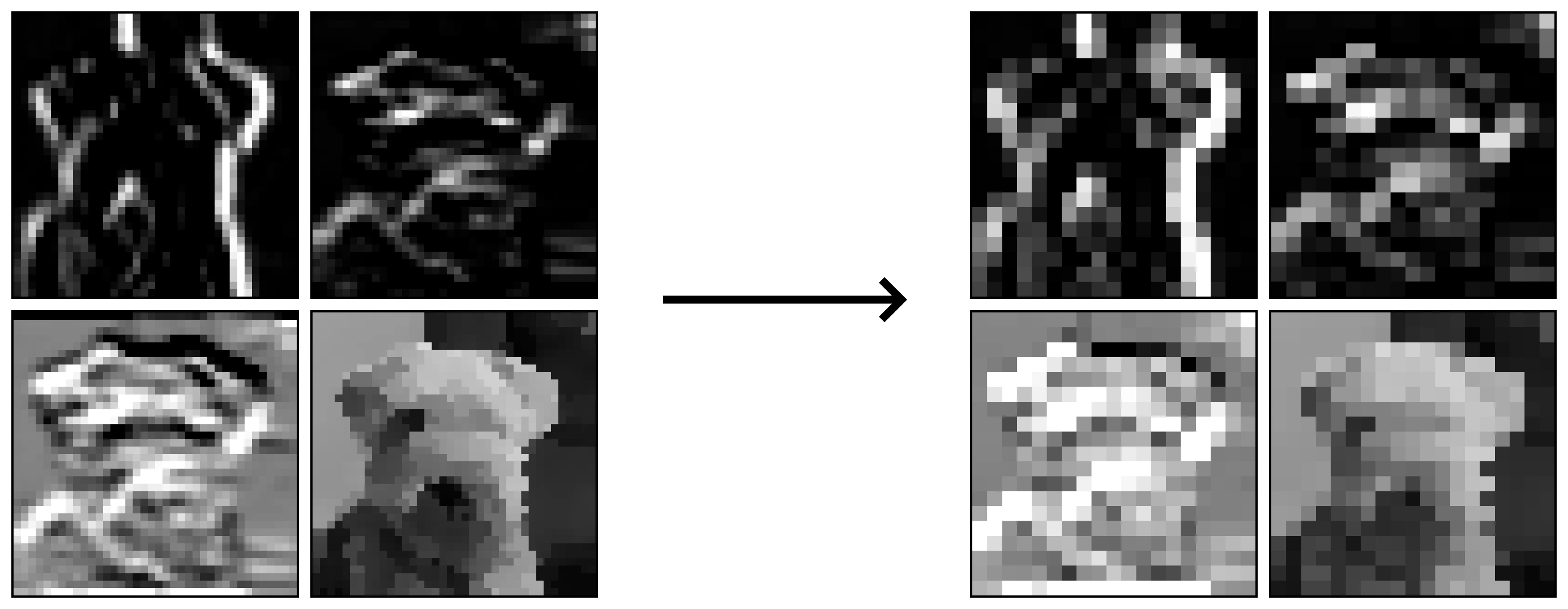
Each convolutional layer has multiple filters, known as kernels, to extract multiple features from the input.
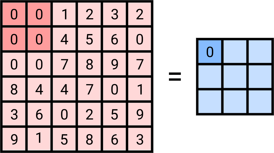
Each kernel slides over the input data and returns a 2D matrix of values called a feature map. To calculate the value of an output neuron, you must multiply each value in its receptive field by the corresponding kernel value, and sum the results. The receptive field is the area which impacts the output of a given neuron, and is the same size as the kernel. Therefore an output neuron can be calculated as the sum of the element-wise multiplication the receptive field and the kernel.
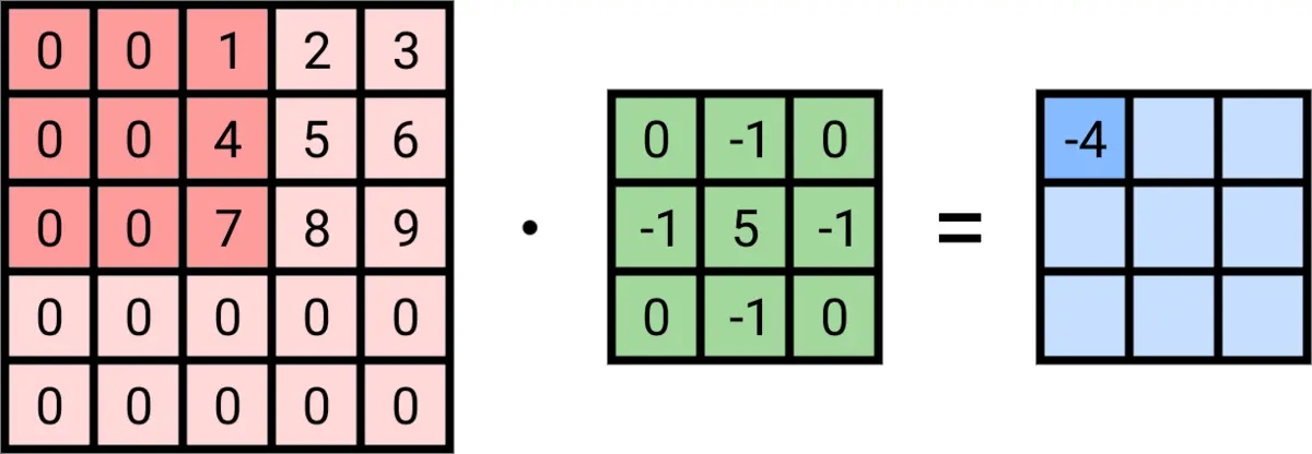
A 3x3 kernel convolves over a 5x5 input, forming a 3x3 output. The receptive field for each output neuron is highlighted in the input matrix. Note that the bias, which is added to each output neuron, is omitted in this example.
A pooling layer acts to reduce the number of parameters in the network, which reduces the complexity of the network. Typically, a pooling layer is placed after each convolutional layer. The standard pooling layer has a 2x2 filter and a stride of 2. Stride is a hyperparameter of both the convolutional layer and pooling layer, and denotes how far the receptive field shifts between each output neuron.
There are two types of pooling layer: average pooling and max pooling. Average pooling takes the mean value of its receptive field, whereas max pooling takes the max value of its receptive field. Max pooling is more commonly used as it reduces the number of parameters which affect the output by 75%, reducing the computation needed for backpropagation.
Max pooling with a 2x2 filter and a stride of 2.
Max pooling layers use the fact that neighbouring pixels are related, and can likely be compressed while not losing the core features of the image. This quality is known as spatial locality and makes CNNs particularly good at processing images when compared to multi-layer perceptrons, which account for each pixel individually.
Max pooling can preserve important parts of the feature maps whilst reducing size by 75%.
Once the network has significantly reduced in size, a regular neural network is used to generate a prediction for classification. The last neurons are flattened and all connected individually to each output neuron, which represent the network's confidence that the image represents each class.
A full convolutional neural network.
Backpropagation starts with the fully connected output layer. The training data used in supervised learning will have a label, which can be used to generate desired outputs.
The fully connected layer backpropagates in the same way as a normal neural network. In this implementation the mean squared error cost function was chosen for simplicity, however in multi-class prediction problems the softmax cost function is usually more appropriate.
Click on a section of the network to backpropagate.
Where \(a^1_2\) represents the second activation on the first layer, \(w\) stands for weight, \(b\) stands for bias, \(y\) stands for the desired value, and \(C\) stands for the cost.
The trick with the max pooling layer is to realise that changes to the neurons which are not the highest output will not have any effect on the cost function, as only the highest output was propagated forward. This makes the backpropagation simple as most of the neurons have 0 error in this layer, and the highest input neurons share the same derivative with the output neurons.
Click on a section of the network to backpropagate. The border of the receptive field is emboldened, and the largest activation in the receptive field is shaded in red.
The convolutional layer has the most complicated backpropagation steps. Convolutions use each kernel parameter and input neuron multiple times in their calculations, so you must find the errors of each output neuron which includes the relevant variable in its calculation.
Click on a section of the network to backpropagate.
A convolutional autoencoder usually uses alternating convolutional and pooling layers in its architecture. Each convolutional layer will have multiple kernels which create multiple feature maps, this allows the model to learn different features of the data more easily. Each of these feature maps will then have a pooling layer applied independently, giving an output of N matrices.
The next layer will be convolutional, but now has an input of N matrices instead of one. Therefore, the kernels in this layer are 3D, and perform element-wise multiplication across the input matrices before taking the sum of the result. This is performed multiple times with multiple 3D kernels to generate feature maps to be fed into the next pooling layer.
Finally, the output is flattened and fully connected to a classification layer, which usually uses the softmax activation function.

Example CNN structure for classifying the MNIST dataset.