Transformers are a type of neural network which are designed for use in natural language processing. They are able to learn long-range dependencies in data, and are used in many state-of-the-art large language models. In this article, I will explain how transformers work and how to build one from scratch for sentiment analysis.
A transformer requires a numerical vector input, so before handling the details of the transformer architecture, we must convert words into meaningful vectors which can be fed into the model.
The simplest way to embed a word into a vector is to use one-hot encoding, where each vector has a single 1 value, with every other value set to 0. The size of the vector is equal to the length of the given dictionary. Despite its simplicity, this isn't a good approach for natural language processing. Transformers scale quickly as you increase the dimensionality of the input embeddings, so a smaller vector is requied. Additionally, one-hot vectors don't give any information about the word it represents. Ideally, we would like vectors where words with similar meanings have similar vectors, whilst occupying a small space. This is known as the semantic space, and is the basis for word embeddings.
A co-occurrence matrix is a simple way to represent the number of times a word appears in the context of another word, and is able to produce a useful vector for natural language problems. The matrix is constructed by counting the words adjacent to each word in a corpus, which gives information about the context each word is used in. For example, in the sentence "the cat sat on the mat", the co-occurrence matrix would be:
| the | cat | sat | on | mat | |
| the | 0 | 1 | 0 | 1 | 1 |
| cat | 1 | 0 | 1 | 0 | 0 |
| sat | 0 | 1 | 0 | 1 | 0 |
| on | 1 | 0 | 1 | 0 | 1 |
| mat | 1 | 0 | 0 | 1 | 0 |
A co-occurrence matrix for the sentence "the cat sat on the mat". "The" is adjacent to "cat", "on" and "mat", so the values in those columns are incremented.
When applied to a large corpus, the co-occurrence matrix provides useful information about the context each word is used in. However, the matrix will be sparse and very large, so it is not suitable to be used as an input to a transformer. To reduce the dimensionality of the matrix, principal component analysis can be applied to the matrix.
Principal component analysis (PCA) is a technique used to reduce the dimensionality of a dataset with minimal loss of information. It works by transforming the data onto a new coordinate system, attempting to represent the data as accurately as possible with fewer dimensions.
To see how PCA works, imagine a 2D dataset with a linear correlation. Two variables are required to describe each data point, however, by transforming the data such that the axes match the direction of the linear correlation, a single variable could adequately describe each point. This is the essence of PCA, and can be applied to datasets with many dimensions. PCA is used to find the directions of maximum variance in the data, called the principal components. These can subsequently be used to reduce the dimensionality of the data.
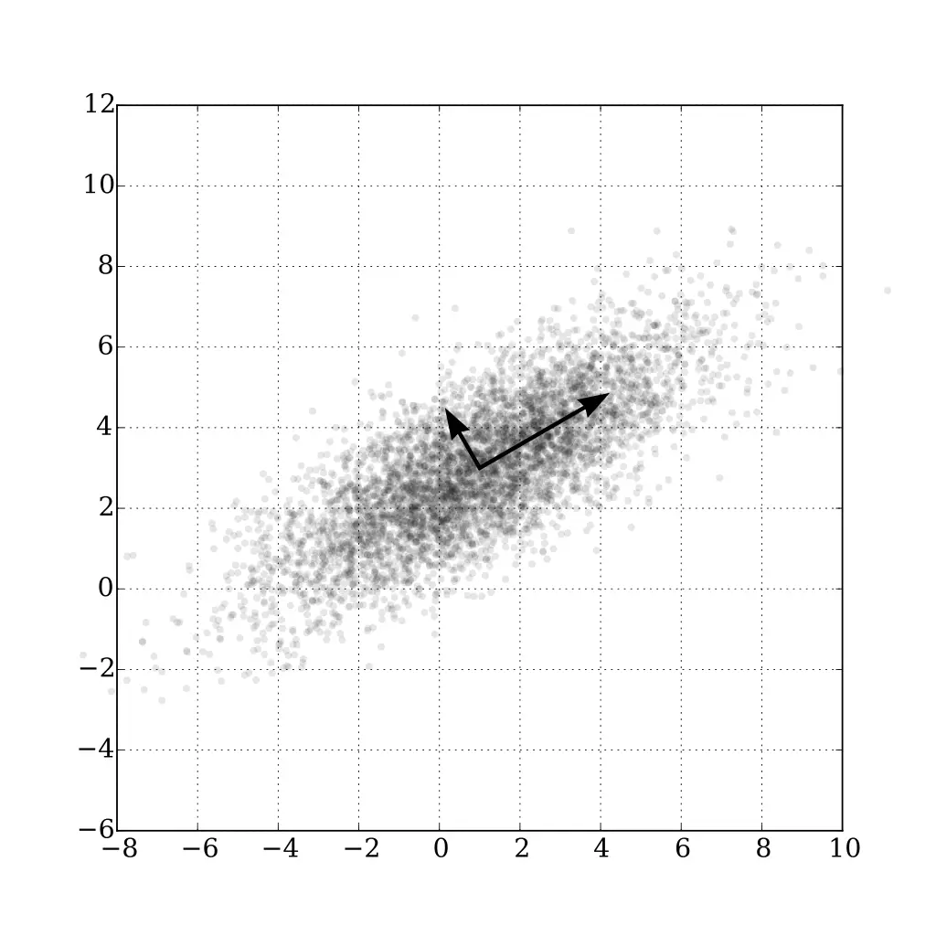
A 2D dataset with a linear correlation and its principal components.
In this example, the points can be adequately described by its largest principal component, which is the direction of maximum variance. When applied to a dataset with many dimensions, PCA can be used to reduce the dimensionality of the data by taking the top principal components.
First, the data must be standardised. This requires subtracting the row mean from each value, and dividing by the row standard deviation. This ensures that each row has a mean of 0 and a standard deviation of 1.
Then, calculate the covariance matrix of the standardized data. The covariance matrix is a square matrix where each value COV(X,Y) represents the covariance between the variables X and Y. The covariance between two variables is a measure of how much they change together. If the covariance is positive, then the variables are positively correlated and vice-versa.
$$ COV(X,Y) = \frac{1}{n} \sum_{i=1}^{n} (x_i - \bar{x})(y_i - \bar{y}) $$
As the mean of each row is 0, this can be simplified to:
$$ COV(X,Y) = \frac{1}{n} \sum_{i=1}^{n} x_i y_i $$
Next, calculate the eigenvectors and eigenvalues of the covariance matrix. The eigenvectors are the directions of maximum variance, and the eigenvalues are the amount of variance in each direction. The eigenvectors are the principal components of the dataset.
A technique to find the eigenvectors and eigenvalues of a matrix is to use the power iteration method. This involves multiplying each row of the matrix by a randomly initialised vector, and normalising the result. This step is repeated by using the output as the vector for the next multiplication. After several iterations, the vector will converge to the eigenvector with the largest eigenvalue.
$$ v_{k+1} = \frac{Av_k}{||Av_k||} $$
To find the other eigenvectors, you can redirect the matrix to remove the largest eigenvector, and repeat the power iteration method. Redirecting the matrix involves the following calculation:
$$ A' = A - \lambda v v^T $$
Where \(A\) is the original matrix and \(v\) is the eigenvector with the largest remaining eigenvalue (\(\lambda\)). By using the power iteration method on the redirected matrix, you can find the eigenvector with the second largest eigenvalue. This can be repeated until the desired number of eigenvectors have been found.
Finally, the original dataset can be transformed by multiplying it by the eigenvectors. This will reduce the dimensionality of the dataset, while retaining as much information as possible. The calculation is as follows:
$$ Y = X V $$
Where \(X\) is the original dataset, \(V\) is the matrix of eigenvectors, and \(Y\) is the transformed dataset.
This reduces the dimensionality of each row to the number of eigenvectors used. The eigenvectors are the principal components of the dataset, and convey the most information about the dataset in the fewest dimensions.
By using PCA on the co-occurrence matrix, each word embedding can be reduced to a manageable size. These embeddings can then be used as the input to a transformer.
A transformer is a neural network architecture that uses attention to excel at natural language processing tasks. It was introduced in the paper Attention is All You Need by Vaswani et al. in 2017.
Transformers are composed of an encoder and a decoder. The architecture is shown in full below:
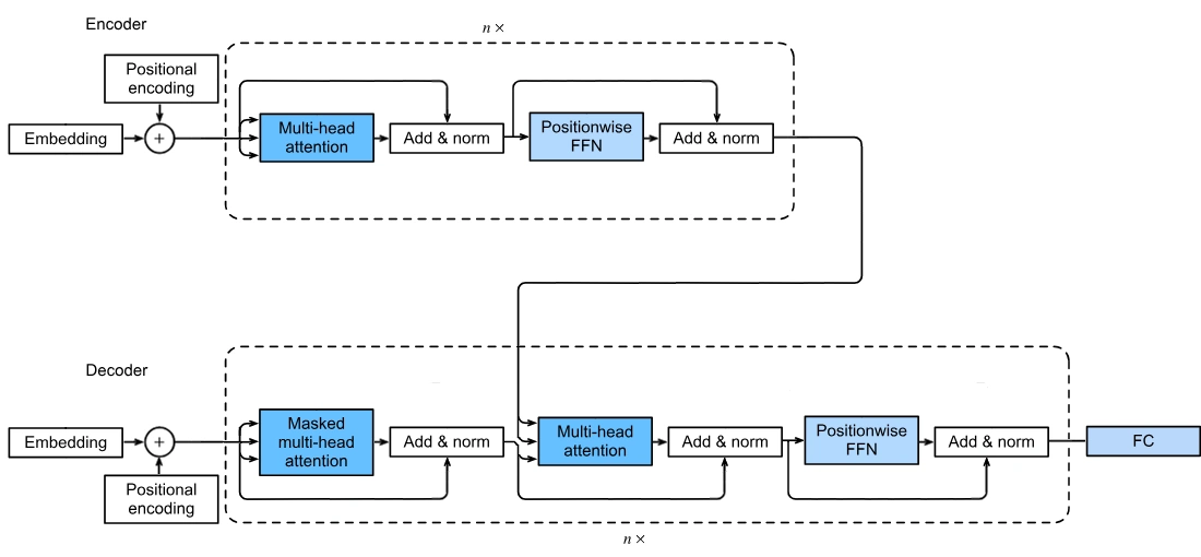
Machine learning models which use transformers usually don't use both the encoder and decoder unless they are performing a translation task. For example, the GPT-3 model only uses the decoder and the BERT model only uses the encoder. In this article, I will focus on an encoder-only transformer.
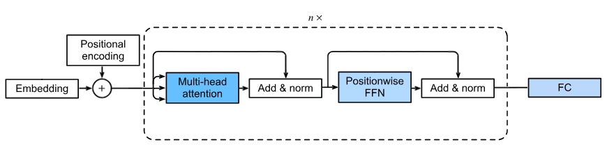
An encoder-only transformer.
Words can have different meanings depending on their position in a sentence. To give the model information about the position of each word, positional encoding is used. This involves adding a vector to each word embedding, which contains information about the position of the word. The positional encoding can use a variety of functions, but the most common is the sine and cosine function:
$$ PE_{(pos, 2i)} = sin(pos / 10000^{2i / d_{model}}) $$
$$ PE_{(pos, 2i+1)} = cos(pos / 10000^{2i / d_{model}}) $$
Where pos is the position of the word, i is the dimension of the embedding, and dmodel is the dimensionality of the embedding. This is the function used in the original paper, and is a good choice for most applications.
$$\begin{bmatrix}0.92 \\ 0.19 \\ 0.39 \\ 0.45 \end{bmatrix} + \begin{bmatrix}\sin (12/10000^{0/4}) \\ \cos (12/10000^{1/4}) \\ \sin (12/10000^{2/4}) \\ \cos (12/10000^{3/4}) \end{bmatrix}$$
An example positional encoding step for a word at position 12.
Self-attention is a technique used to find the relationship between each word in a sentence. For example in the sentence "Alice threw Bob her phone", the model requires context from "Alice" and "her" to determine the owner of the phone. Therefore, the model attempts to determine which words are relevant to each other, or the 'attention' each word should pay to the others.
To accomplish this, the model calculates a weight for each pair of words. This weight intends to represent the importance of the first word to the second. The weights are calculated by finding the dot product of the pair.
$$ W_{n,m} = V_n \cdot V_m $$
Where Vn is the nth word embedding, and Wn,m is the weight between the nth and mth word.
These weights are then normalised for each row using the softmax function, which ensures that the sum of the weights for each word is 1.
$$ W_{n,m} = \frac{e^{W_{n,m}}}{\sum_{i=1}^{n} e^{W_{n,i}}} $$
Then, a new vector is calculated for each word by multiplying a word embedding by its respective weight and summing the resulting vectors.
$$ V_{n} = \sum_{i=1}^{n} W_{n,i} V_{i} $$
This process helps the model to understand the relationship between each word in a sentence. However, the model currently has no control over the output of the self-attention layer. To give the model more control and allow it to learn the relationships between words, key, query, and value matrices are added as parameters.
When you multiply a 1xN vector by an NxN matrix, you get a 1xN vector. Due to this, the key, query, and value matrices are NxN matrices, where N is the dimensionality of the word embeddings. The word embeddings are used in three places in the self-attention step, known as the key, query, and value. This is where the new matrices are applied to the model, to give the model control of the output. This gives new equations for the weights and output vectors:
$$ W_{n,m} = V_n \times M_K \cdot V_m \times M_Q $$
$$ V_{n} = \sum_{i=1}^{n} W_{n,i} V_{i} \times M_V $$
Where MK, MQ, and MV are the key, query, and value matrices respectively.
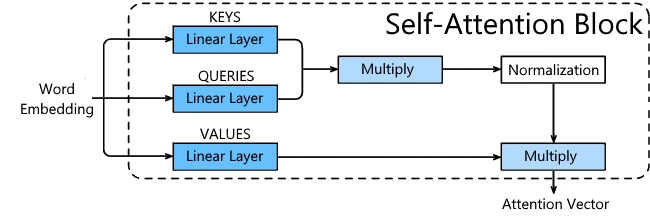
The architecture of a self-attention block.
Multi-head attention is a technique used to improve the performance of self-attention. It involves using multiple self-attention blocks, resulting in multiple key, query, and value matrices. Then, the output of each self-attention block is concatenated and fed into a linear layer. A linear layer can be implemented as a fully connected layer without an activation function. This allows the model to learn different relationships between words.
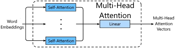
The architecture of a multi-head attention block.
After the self-attention block, the output is added to the residual input and normalised. This step helps stabilize the training process. The normalization is done using layer normalization, which normalizes across the features, rather than across the batch. This means that if the dimensionality of the word embeddings was 200, the mean and standard deviation would be calculated over the 200 dimensions for each row.
The positionwise feed-forward network is a fully connected layer, usually using a ReLU activation function. The output of the layer is the same dimensionality as the input. For more information on feed-forward neural networks, see my article on them.
Lastly, the residual input is added to the output of the positionwise FFN and normalised using layer normalization.
The encoder uses a stack of N identical sections, each containing a multi-head attention block, add & norm, positionwise FFN and another add & norm. Finally, you must reduce the dimensionality of the output using a linear layer to get your final output. For sentiment analysis, the output is a single value, so the linear layer output is a single neuron. For text generation, the output is a vector of probabilities for each word in the vocabulary.
This is everything you need to know about the forward propagation of an encoder-only transformer. Once forward propagation is complete, you can use backpropagation with a desired sentiment or word to train the model.
Backpropagation computer gradients for the model in reverse, calculating the gradient of each parameter with respect to the cost function. The gradient is then used to update the parameters using gradient descent.
For more information on the gradient descent algorithm, and the backpropagation for fully connected and linear layers, see my article on neural networks.
The backpropagation for the add & norm block is deceptively difficult. This is due to the numerous uses of each input in the forward propagation. However, as the block has no parameters, the adjustment step can be skipped.
The forward propagation for the add & norm block is:$$ \frac{(x_1 + x_2) - \mu}{\sigma} $$
Where \(x_1\) is the residual input, \(x_2\) is the output of the previous block, and \(\mu\) and \(\sigma\) are the mean and standard deviation of the output of the self-attention block respectively.
It is fairly trivial to see that \(x_1\) and \(x_2\) will share the same gradient, as if the gradient of \(x_1 + x_2\) with respect to the cost function is positive, the gradient of \(x_1\) and \(x_2\) must also be positive.
Therefore, we need to backpropagate the following:
$$ \frac{x - \mu}{\sigma} $$
If you imagine a dimensionality of 2 for the word embeddings, you can expand this to:
$$ \frac{\begin{pmatrix}x_1 \\ x_2\end{pmatrix} - \frac{x_1+x_2}{2}}{\frac{(x_1 - \frac{x_1+x_2}{2})^2 + (x_2 - \frac{x_1+x_2}{2})^2}{2}} $$
It's now clear to see why backpropagating with respect to each input is difficult.
The exact steps of differentiating the above equation are beyond the scope of this article, but the details can be found in this article [arch.]. The final result is:
$$ J = \frac{N * I - 1}{N \sigma} - \frac{(x - \mu) \odot (x - \mu)^T}{N \sigma ^ 3}$$
Where \(N\) is the dimensionality of the input, \(I\) is the identity matrix, \(\sigma\) is the standard deviation of the input, \(x\) is the input, and \(\mu\) is the mean of the input.
This gives us the Jacobean matrix \(J\) to pass to the previous block. The Jacobean matrix is a matrix of partial derivatives, where each row is the gradient of the output with respect to each input.
The backpropagation for the multi-head attention block is fairly simple. Firstly, backpropagate the linear layer. Then, backpropagate each head individually. Finally, sum the gradients of each head and backpropagate to the previous block.
Firstly, we must find the rate of change of the output with respect to each element in the value matrix. In a scenario with 2 words and 3 dimensions, we have:
$$ \begin{pmatrix}w_{11} & w_{12} & w_{13} \\ w_{21} & w_{22} & w_{23}\end{pmatrix} \cdot \begin{pmatrix}v_{11} & v_{12} & v_{13} \\ v_{21} & v_{22} & v_{23} \\ v_{31} & v_{32} & v_{33}\end{pmatrix} = \begin{pmatrix}y_{11} & y_{12} & y_{13} \\ y_{21} & y_{22} & y_{23}\end{pmatrix} $$
Now, for each element in the value matrix, we can calculate the rate of change of the output with respect to that element by finding all of its uses in the output matrix. For example, for \(v_{11}\), we have:
$$ y_{11} = w_{11}v_{11} + w_{12}v_{21} + w_{13}v_{31} $$ $$ \frac{\partial y_{11}}{\partial v_{11}} = w_{11} $$
$$ y_{21} = w_{21}v_{11} + w_{22}v_{21} + w_{23}v_{31} $$ $$ \frac{\partial y_{21}}{\partial v_{11}} = w_{21} $$
$$ \frac{\partial C}{\partial v_{11}} = w_{11} \cdot \frac{\partial C}{\partial y_{11}} + w_{21} \cdot \frac{\partial C}{\partial y_{21}} $$
Then, we need to find the rates of change for each \(w_{ij}\). For example, for \(w_{11}\), we have:
$$ y_{11} = w_{11}v_{11} + w_{12}v_{21} + w_{13}v_{31} $$ $$ \frac{\partial y_{11}}{\partial w_{11}} = v_{11} $$
$$ y_{12} = w_{11}v_{12} + w_{12}v_{22} + w_{13}v_{32} $$ $$ \frac{\partial y_{12}}{\partial w_{11}} = v_{12} $$
$$ y_{13} = w_{11}v_{13} + w_{12}v_{23} + w_{13}v_{33} $$ $$ \frac{\partial y_{13}}{\partial w_{11}} = v_{13} $$
$$ \frac{\partial C}{\partial w_{11}} = v_{11} \cdot \frac{\partial C}{\partial y_{11}} + v_{12} \cdot \frac{\partial C}{\partial y_{12}} + v_{13} \cdot \frac{\partial C}{\partial y_{13}} $$
Now we have the error of each weight, so we can start backpropagating the softmax normalisation step. The steps are outside of the scope of this article, but the details can be found here [arch.].
The result gives two different cases:
$$ w_{ij} = \frac{e^{x_{ij}}}{\sum_{k=1}^{n} e^{x_{ik}}} $$
$$\text{if } j = k $$ $$ \frac{\partial w_{ij}}{\partial x_{ik}} = w_{ij}(1 - w_{ij}) $$
$$\text{if } j \neq k $$ $$ \frac{\partial w_{ij}}{\partial x_{ik}} = -w_{ij}w_{ik} $$
$$ \frac{\partial C}{\partial x_{ij}} = \sum_{k=1}^{n} \frac{\partial C}{\partial w_{ik}} \cdot \frac{\partial w_{ik}}{\partial x_{ij}} $$
Now, with the Jacobean matrix for the softmax normalisation step, we can backpropagate the error to the multiplication step. To find \(x_{ij}\), we used:
$$ x_{ij} = \begin{pmatrix}a_{i,1} \\ a_{i,2} \\ a_{i,3}\end{pmatrix} \cdot \begin{pmatrix}b_{j,1} \\ b_{j,2} \\ b_{j,3}\end{pmatrix}$$
Where \(a_{i}\) is the \(i\)th input embedding multiplied by the query matrix, and \(b_{j}\) is the \(j\)th input embedding multiplied by the key matrix. We can find the error of each of these as follows:
$$ \frac{\partial C}{\partial a_{ik}} = \sum_{j=1}^{n} \frac{\partial C}{\partial x_{ij}} \cdot \frac{\partial x_{ij}}{\partial a_{ik}} $$
$$ = \sum_{j=1}^{n} \frac{\partial C}{\partial x_{ij}} \cdot b_{jk} $$
The same process can be applied to \(b_{j}\). Then, we can find the error of the query matrix as follows:
$$ a_{i} = \begin{pmatrix}e_{i,1} & e_{i,2} & e_{i,3}\end{pmatrix} \cdot \begin{pmatrix}q_{11} & q_{12} & q_{13} \\ q_{21} & q_{22} & q_{23} \\ q_{31} & q_{32} & q_{33}\end{pmatrix}$$
$$ \frac{\partial C}{\partial q_{ij}} = \sum_{k=1}^{n} \frac{\partial C}{\partial a_{kj}} \cdot \frac{\partial a_{kj}}{\partial q_{kj}} $$
$$ = \sum_{k=1}^{n} \frac{\partial C}{\partial a_{kj}} \cdot e_{kj} $$
An identical process can be applied to the key matrix:
$$ \frac{\partial C}{\partial k_{ij}} = \sum_{k=1}^{n} \frac{\partial C}{\partial b_{kj}} \cdot e_{kj} $$
Finally, we can find the error of the input embeddings:
$$ \frac{\partial C}{\partial e_{ij}} = \sum_{k=1}^{n} \left( \frac{\partial C}{\partial a_{kj}} \cdot \frac{\partial a_{kj}}{\partial e_{ij}} + \frac{\partial C}{\partial b_{kj}} \cdot \frac{\partial b_{kj}}{\partial e_{ij}} \right)$$
$$ = \sum_{k=1}^{n} \left( \frac{\partial C}{\partial a_{kj}} \cdot q_{ik} + \frac{\partial C}{\partial b_{kj}} \cdot k_{ik} \right)$$
This step is the most challenging to understand due to the number of calculations involved. However, by carefully splitting the problem into steps, each derivation is relatively simple. An example implementation of the self-attention backpropagation can be found on my GitHub.
All components of the encoder-only transformer are now fully backpropagated. This allows us to train the model using gradient descent, and the model will slowly learn our desired output with enough training examples.
Note: the positional encoding step is not backpropagated, as there are no trainable parameters.
These are all of the necessary elements needed to build a transformer from scratch. Transformers are a powerful tool for natural language processing, and can be trained to perform sentiment analysis, machine translation, and many other tasks. The transformer architecture is also the basis for the GPT models, which are currently the state-of-the-art for natural language processing.
I have implemented an encoder-only transformer in Rust for sentiment analysis, and the code can be found on my GitHub below. It's important to note that training a transformer is a difficult task, as described here. This means that the performance of a transformer implemented from scratch is unlikely to match that of a transformer implemented in a framework providing cutting-edge optimisation and training techniques. Therefore, for real-world applications it's usually more suitable to use a machine learning library such as TensorFlow.
However, I hope that this article has provided a useful introduction to the transformer architecture, and that it has helped to demystify the inner workings of transformers.
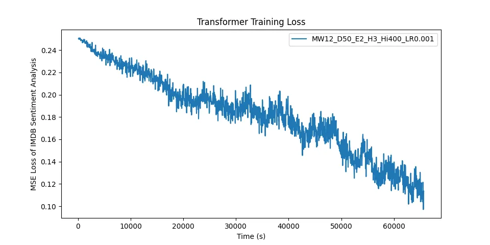
Loss of my RustTransformer model over time when training on this dataset of polarised movie reviews.
This specific model was trained with 12 words & 50 dimensions per sample, 2 encoder blocks, 3 attention heads, a hidden layer size of 400 and a learning rate of 0.001.